

在数据分析和机器学习领域,聚类作为一种核心技术,对于从未标记数据中发现模式和洞察力至关重要。聚类的过程是将数据点分组,使得同组内的数据点比不同组的数据点更相似,这在市场细分到社交网络分析的各种应用中都非常重要。然而,聚类最具挑战性的方面之一在于确定最佳聚类数,这一决策对分析质量有着重要影响。
虽然大多数数据科学家依赖肘部图和树状图来确定K均值和层次聚类的最佳聚类数,但还有一组其他的聚类验证技术可以用来选择最佳的组数(聚类数)。我们将在sklearn.datasets.load_wine问题上使用K均值和层次聚类来实现一组聚类验证指标。以下的大多数代码片段都是可重用的,可以在任何数据集上使用Python实现。
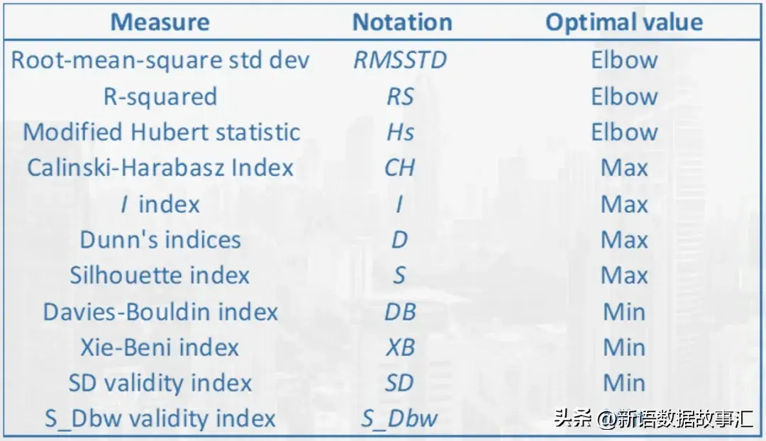
接下来我们主要介绍以下主要指标:
Gap统计量(Gap Statistics)(!pip install --upgrade gap-stat[rust])
Calinski-Harabasz指数(Calinski-Harabasz Index )(!pip install yellowbrick)
Davies Bouldin评分(Davies Bouldin Score )(作为Scikit-Learn的一部分提供)
轮廓评分(Silhouette Score )(!pip install yellowbrick)
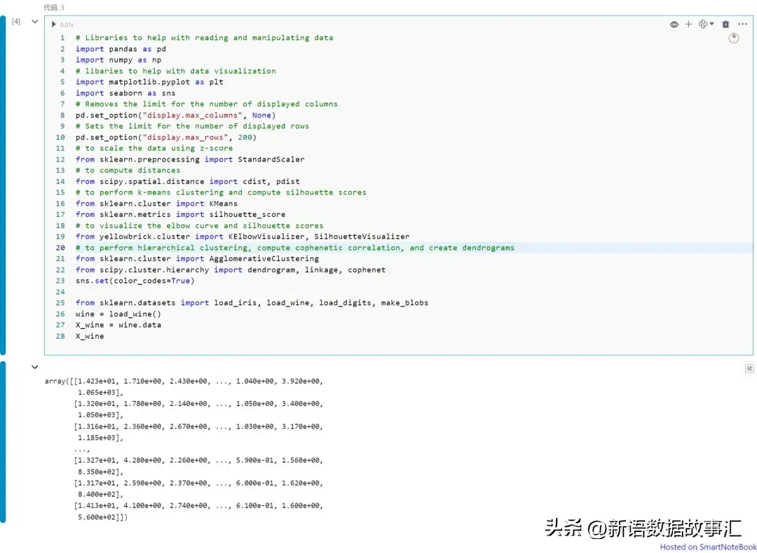
引入包和加载数据
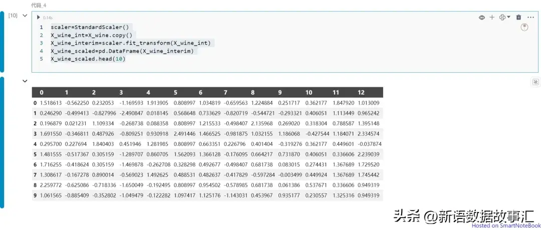
标准化数据:
Gap统计量(Gap Statistics)
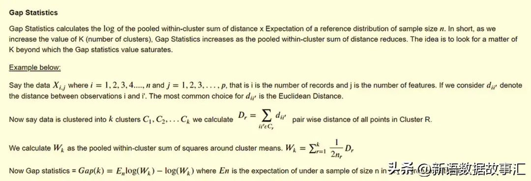
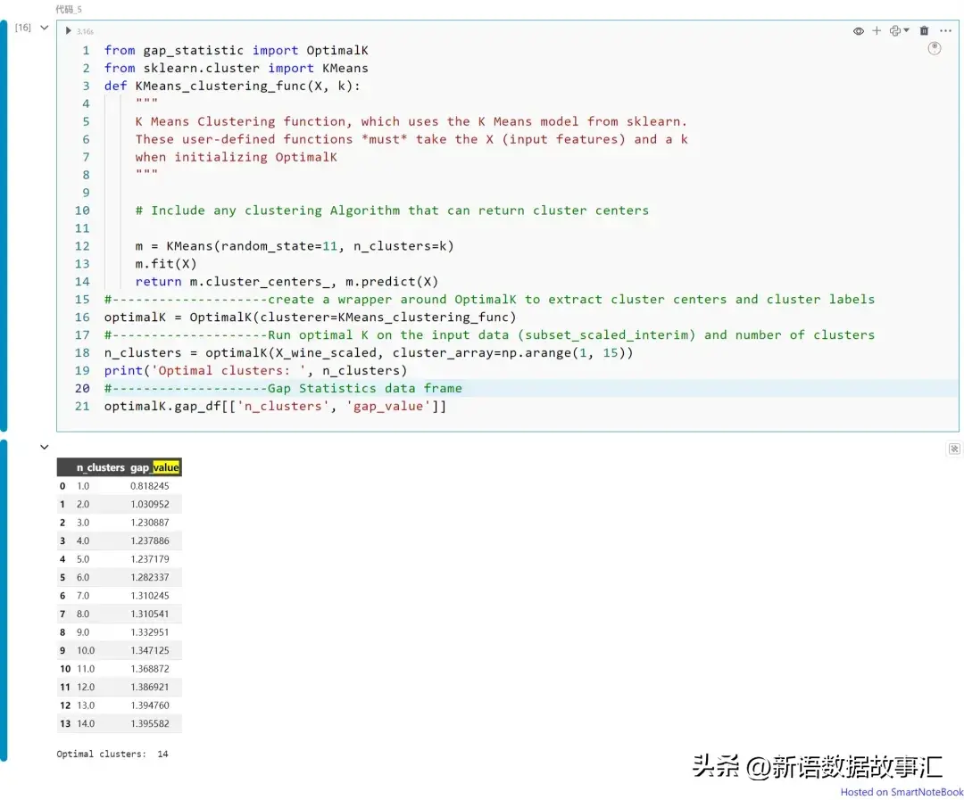
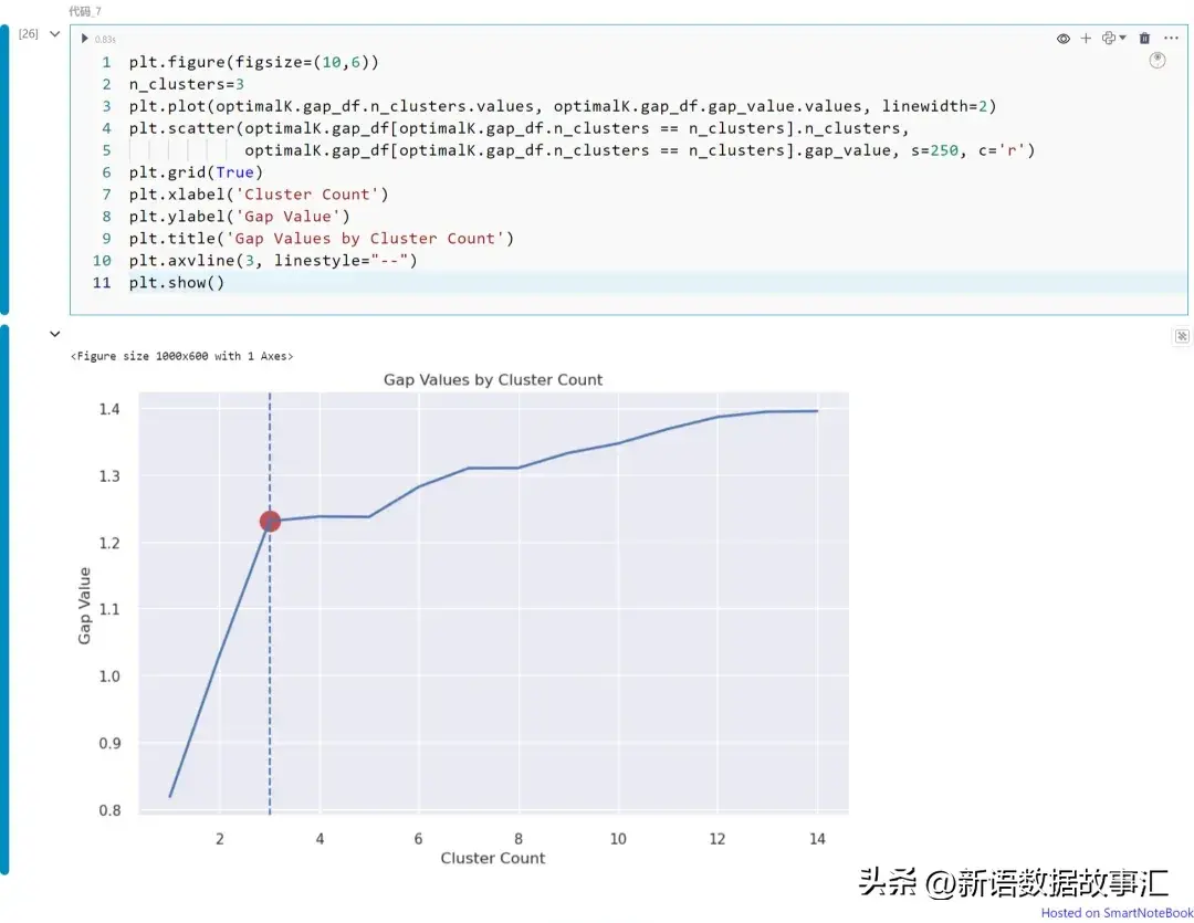
上图展示不同K值(从K=1到14)下的Gap统计量值。请注意,在本例中我们可以将K=3视为最佳的聚类数。如上所述,可以从图中获得Gap统计量的拐点。
Calinski-Harabasz指数(Calinski-Harabasz Inde)
Calinski-Harabasz指数,也称为方差比准则,是所有组的组间距离与组内距离之和(群内距离)的比值。较高的分数表示更好的聚类紧密度。可以使用Python的YellowBrick库中的KElbow visualizer来计算。
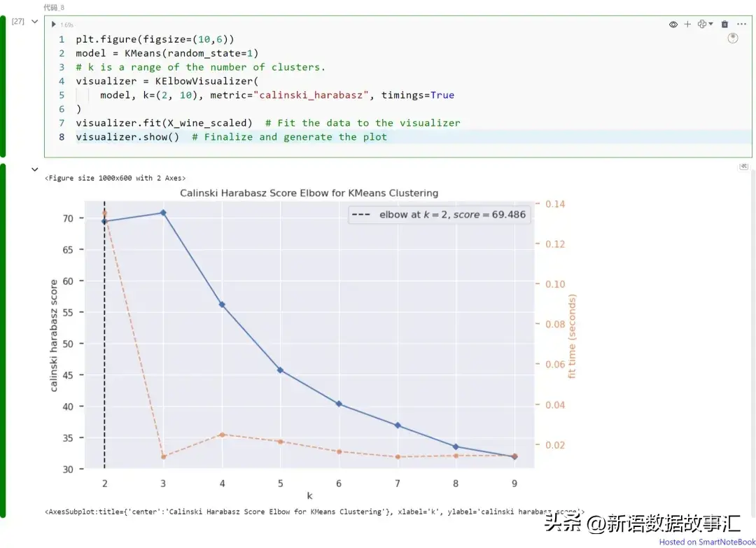
上图展示不同K值(从K=1到9)下的Calinski Harabasz指数。请注意,在本例中我们可以将K=2视为最佳的聚类数。如上所述,可以从图中获得Calinski Harabasz指数的最大值。
使用“metric”超参数选择用于评估群组的评分指标。默认使用的指标是均方失真,定义为每个点到其最近质心(即聚类中心)的距离平方和。其他一些指标包括:
distortion:点到其聚类中心的距离平方和的均值
silhouette:聚类内距离与数据点到其最近聚类中心距离的比率,对所有数据点求平均
calinski_harabasz:群内到群间离散度的比率
Davies-Bouldin指数(Davies-Bouldin Index)
Davies-Bouldin指数计算为每个聚类(例如Ci)与其最相似聚类(例如Cj)的平均相似度。这个指数表示聚类的平均“相似度”,其中相似度是一种将聚类距离与聚类大小相关联的度量。具有较低Davies-Bouldin指数的模型在聚类之间有更好的分离效果。对于聚类i到其最近的聚类j的相似度R定义为(Si + Sj) / Dij,其中Si是聚类i中每个点到其质心的平均距离,Dij是聚类i和j质心之间的距离。一旦计算了相似度(例如i = 1, 2, 3, ..., k)到j,我们取R的最大值,然后按聚类数k进行平均。
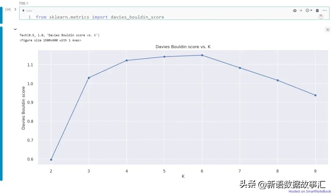
上图展示不同K值(从K=1到9)下的Davies Bouldin指数。请注意,在本例中我们可以将K=2视为最佳的聚类数。如上所述,可以从图中获得Davies Bouldin指数的最小值,该值对应于最优化的聚类数。
轮廓分数(Silhouette Score)
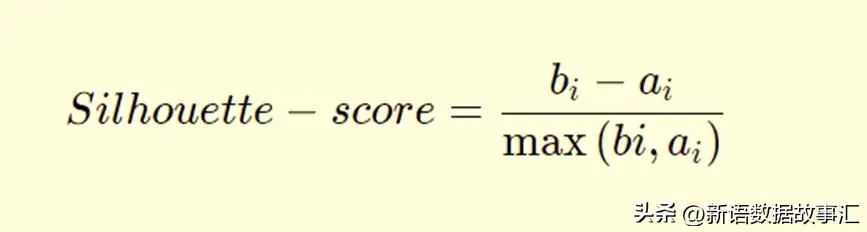
轮廓分数衡量了考虑到聚类内部(within)和聚类间(between)距离的聚类之间的差异性。在下面的公式中,bi代表了点i到所有不属于其所在聚类的任何其他聚类中所有点的平均最短距离;ai是所有数据点到其聚类中心的平均距离。如果bi大于ai,则表示该点与其相邻聚类分离良好,但与其聚类内的所有点更接近。
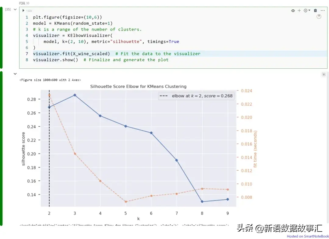
上图展示不同K值(从K=1到9)下的轮廓分数。请注意,在本例中我们可以将K=2视为最佳的聚类数。如上所述,轮廓分数可以从图中获得最大值,该值对应于最优化的聚类数。
在数据分析和机器学习中,聚类是一项关键技术,帮助我们从未标记的数据中发现模式和洞察。确定最佳聚类数是聚类过程中的重要挑战,影响分析质量。本文介绍了多种聚类验证技术如Gap统计量、Calinski-Harabasz指数、Davies Bouldin指数和轮廓分数,这些指标可以帮助我们选择最优化的聚类数,提升聚类结果的有效性和可靠性。


还没有评论,来说两句吧...